When balancing a rotor, we correct its mass distribution in the correction planes by marking it with the PK symbol. The amount of mass and the seating angles of the correction weights are calculated using data from measurements made in the measuring planes, which are marked with the PP symbol. The measuring planes are identification planes.
Three ways to identify unbalance
There are a few ways that practitioners can identify unbalance, including:
a) simplified, which is performed in one measuring and correction plane;
b) total, which is performed simultaneously in two planes;
c) special, which is performed in multiple planes.
Overall, unbalance is identified indirectly. Uncompensated inertial forces that occur at various (unidentified) locations along the length of the rotor either cause it to move or induce forces in support. The motion in supercritical and self-bearing balancers or the forces in subcritical balancers are then calculated in the measuring planes.
The number of measuring and correction planes depends mainly on the stiffness of the rotor. Identification types a) and b) are most common for balancing rigid rotors, and type c) is most common for flexibly prone rotors.
The balancing result depends on the number of measurement planes used. This means that the balancing of a rigid rotor, calculated based on identification in one correction plane, will end up with a different result than that obtained with identification in two measurement planes.
When balancing flexibly prone rotors, only inertia forces are identified (their individual effect on motion). Moments, or the effect of moments from inertia forces on motion, are not identified.
Why discs push you toward a single plane
Caution should be exercised when balancing disks. Because of the impossibility of correcting in two planes far apart along the axis of rotation, practice encourages the use of balancing in a single plane.
The correct procedure for balancing discs is to determine both components of unbalance – force and moment – and then get rid of only the one that can be physically eliminated. This is the force component, called static. To do this, it is necessary to use the identification of motion or force in two measurement planes. On this basis, the machine’s calculation system will determine both components of unbalance. Only after comparing the values of the components with the limits should a correction be made to the force component to eliminate it. The moment component remains on the discs, having acceptable values; if the moment component is greater than acceptable, the selected disc is a deficiency.
If only one plane is identified, the calculation system will not distinguish between the force component and the force belonging to the moment component. All forces acting on this plane are identified. One of the forces forming a pair of forces in the moment component of the unbalance, which occurs in addition to the static component, is also taken into account. As a result of the correction of the mass distribution in this plane, movement and forces in the location and direction of the sensor are completely eliminated. In this way, the simplified balancing procedure completely eliminates vibration in the location and direction of the vibration sensor.
What single-plane correction leaves behind
Because of the single-plane identification, the values of these parameters at other support points, on the axis of rotation, may increase with distance from the sensor axis. Thus, the remaining moment component affects other components of the rotating machine structure. This is shown in Figure 1, where the center of oscillation S1 has moved to S2, as a result of one-plane balancing. One of the forces F, belonging to the force pair, adds to the resultant acting in the other support of the machine. Although both forces F, forming a pair of forces, lie in one plane, the “addition” of the force to the forces lying in the other plane, does not take place in a ratio of 1:1. Usually a part of the force F is added. This is used in practice. By repeated single-plane balancing, alternating left and right, the process converges to a residual value.
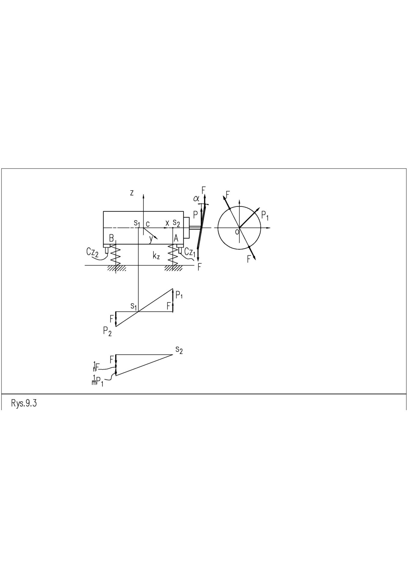
In practice, simplified balancing guarantees “smooth” operation of a rotating machine when the level of vibration or force on the opposite support is simultaneously checked on the balancing machine or after an additional condition concerning the radial “run-out” of the rotor, which is most often in the form of a disc.
Fewer measurements, faster convergence
Thus, it is a balancing that does not cover the entire unbalance. Its advantage over balancing in two correction planes is the small amount of data needed to perform it. This is particularly important when balancing in self-bearing.
When choosing single-plane balancing, as opposed to two-plane balancing, the advantage of the small amount of data taken from measurements is due to errors, which are distorted measurements. Errors arise from all sorts of conditions, such as the influence of vibrations from the environment, air pumping resistance, drive belt vibrations, clearances in the connection to the cardan shaft, temperature changes and tp. Through the accumulation of measurement errors, the convergence of simplified balancing is better than total balancing. In the zero balancing stage, two data sets are collected: the value of signal amplitude and phase.
In the first stage, four data sets are taken:
a) the value of signal amplitude and phase,
b) the value of the mass and the angle of foundation of the test weight.
When balancing in two planes, 16 measurements are taken.
Simplified balancing (where four data points are taken) gives a quick answer. In the presence of large disturbances, simplified balancing in several steps converges faster than total balancing in one step.
Single-step balancing is used for balancing flexibly prone rotors when minimizing the deflection of the first modal form (that is, in the shape of half of a sine wave). The methods adopted in practice—coefficients and modal, balancing flexibly prone rotors—do not identify moments from forces. By this, taking PP=PK=1 is an obvious action.
The support point of, for example, a process shaft on which the disc is mounted, must be sensed in such a way that it is possible to measure the values of the amplitude and phase of the sensor signal, relative to the pitch associated with the rotor. The pitch on the rotor, while spinning, must increase relative to the blade (this is a necessary condition).
Choosing the measuring plane and mounting the sensor
In preparation for balancing, it is necessary to determine the place where the sensor will be mounted and the motion or force data will be collected (in the form of a motion or force transducer to an electrical signal), called the measuring point or plane. It is perpendicular to the axis of rotation. On a balancing machine, the sensor is mounted to a support. The axis of the sensor must intersect the axis of spinning — it does not have to be located along the length of the rotor and can also lie outside its span. It is only important that the mounting location of the sensor is unambiguously (reproducibly) connected to the rotor support structure. As a result of incorrect attachment of the sensor, for example, foundation with slack or through an intermediate element showing susceptibility to force, an additional vibration system will be created at the place of its attachment. Because of this, the measurement results will be “disturbed” by its influence. This “disturbance” will not affect the result if it remains invariant in the sense that it is repeatable at each rotation engagement, and repeatability is understood as invariant dynamic properties.
Choosing the correction plane
It is necessary to determine the place where the test and correction weights will be attached, called the point or plane of correction. On subcritical balancers, the mounting locations of correction weights are selected according to technological needs and without restrictions. Test weights are not used at all. Enabling decoupling of the positions of the test and correction planes is due to the lack of oscillatory motion of the entire rotor on the balancer. When balancing in on bearings and supercritical balancers, the mounting locations of test and correction weights are in the same PK. This condition is due to the presence of oscillating motion of the entire rotor. No other restrictions are imposed on the distribution of PP and PK along the length of the rotor. Such a procedure is called the adoption of the distribution of test and correction planes.
Subcritical machines: why no separate calibration is needed
The motion of the rotor, seated on a subcritical balancing machine, is sufficiently approximate to a rotary motion. By meshing the machine, force measurements can be taken, once per revolution, at the same angular position of the rotor relative to the sensor. Therefore, the rotor is “seen” by the machine as not moving. Such a state is called kinetostatic. As a result of rotational motion, the inertia forces from the entire rotor mass cancel each other wherever the rotor is circularly symmetrical. Only the forces from unbalance remain uncompensated. These forces have a constant angular position relative to the rotor. The absence of uncompensated inertia forces from the entire rotor mass makes it possible to decouple the test planes from the correction planes. Therefore, the use of this type of machine does not require a separate calibration for balancing a new rotor. The test weight was already used by the machine manufacturer for the first, universal calibration.
In order to balance a disc, for example, on a subcritical balancing machine with a vertical axis of rotation, it is enough to mount the disc in a chuck and take the required measurements (such as the height of the mounting relative to the spindle and the diameter on which the correction will take place). Then, select the option to divide the unbalance into force and torque components, for example, the diameter and permissible depth of the correction drilling, and then the type of disc size (if the machine has such an option) and press the “Start” button. The machine will give the correct answer, as it is factory-equipped with a calibration module that will assign the unbalance (in the form of the calculated weight of the correction weights) according to the measurement results.
Supercritical machines: calibrating with a test weight
To balance a rotor, for example, on a supercritical, universal and horizontal machine, it is necessary to perform an additional calibration of the vibration system. The only exception is if a rotor of the same mass and identical shape was previously balanced and the calibration was stored in the machine’s memory. As in sub-critical balancing machines, the machine is so orchestrated that vibration measurement is performed, once per rotor rotation, at the same angular position of the rotor relative to the sensor. Due to the high susceptibility of supporting the rotor horizontally, the entire mass of the rotor, in addition to its rotational motion, performs a vibrating motion in the plane. This means it has two degrees of freedom, and inertial forces are generated across the rotor mass. Calibration involves determining the dynamic response of the mechanical system to an external forcing and storing it in memory for use in machine settings. This forcing is a calibration (test) weight attached to the rotor only for the duration of the test. The angle of attachment can be arbitrary. The angle and weight of the load are stored in the machine’s memory and used in calculations. By measuring the amplitudes and phases of the selected vibration parameter, in the band corresponding to the rotor speed, data is obtained for calculating the dynamic response of the mechanical system of the supported rotor to the external forcing, as well as the value and angular position of the unbalance. The identification only concerns the location and direction of the vibration sensor.
The balancing procedure will be shown in detail below. In the background of these considerations, a rotor is supported in two places (on any mechanical stand capable of driving the rotor), sensed to read the amplitude and phase values of a minimum signal from a single sensor. The mechanical system supporting the rotor “converts” an external forcing, which for the rotor is unbalance, into a motion or force. This “transformation” is shown here in the form of a so-called single-plane calibration vector. The vector represents how to “transform” the parameters of a test force located near the sensor, for example, into motion at the location and direction of this sensor.
In the case of two-plane balancing of a rigid rotor, we will learn a different type of calibration coefficients, which will also describe how the motion along the length of the rotor is “transmitted.”
The influence coefficient method
The influence coefficient method is used in balancing machines. In the process of single-plane balancing, the values of two discriminants are sought:
a – the single-plane calibration vector,
Ň0 – the unbalance vector.
Balancing consists of a measurement part and a calculation part. The measuring part comprises zero and first stages. In the zero stage, the rotor is loaded with the original unbalance. In the first stage, the disc is additionally loaded with a test load. Maintaining the same rotor speed, in both stages, ensures unchanged dynamic properties of the mechanical system, including identical susceptibility to external loading.
The entire balancing process, using the coefficient method, includes calibration with a test weight as described below. After the calibration, these coefficients can be saved for use in the next balancing with the same movement conditions.
Balancers measure a selected vibration parameter, such as acceleration, velocity, deflection or force. All these parameters have a similar time course. In the following, we will often refer to these parameters collectively as deflection.
Figure 2 shows the forcing condition, which is associated with the rotor, and the deflection condition, which is associated with the support structure.
The rotor is loaded by:
a) in the zero stage: the inertia force coming from the unbalance Ň0,
b) in the first stage: the inertia force coming from the unbalance + the inertia force coming from the test weight Ň0, Mtest.
It is irrelevant to the final result that the shaft deflects and the sensor is attached to a susceptible support. All that matters is that its susceptibility to deflection will be the same in both balancing stages and its characteristics are linear. The advantage of this method is that the dynamic properties of the system are lumped into a “common bag,” which we can call the dynamic susceptibility at the point and direction of the main axis of the vibration transducer (sensor).
Included in the name of the coefficient method is the method of searching for unbalance. The method introduces the concept of coefficients, which determines the effect of a forcing located at a selected point on the rotor (which is an unbalance) with the motion or forces acting at any point elsewhere in the structure supporting the rotor. The number and type of coefficients depends on the number of adopted planes PP and PK.
The susceptibility coefficient
In single-plane balancing, there is one coefficient, which can be called the susceptibility coefficient. It can be called the susceptibility coefficient. On the balancer, it describes how the support reacts, at the place and direction of attachment of the vibration sensor, to the external forcing. This is the appearance of deflection (vibration or force), at a frequency corresponding to the rotation of the disc, with an amplitude directly proportional to the external forcing and a well-defined phase. The amplitude and phase of these deflections have values specific to the current rotational speed. They are not linearly dependent on the value of the rotational speed.
If balancing is not carried out on a specially prepared test bench, but in a rotating machine and in its own bearings, the phase is determined not only due to the dynamic properties of the rotor support (see the position on the amplitude-phase characteristics), but also based on the geometric summation of vibrations in the selected direction. These vibrations can originate from the several degrees of freedom that a rotor support can have in a rotating machine.
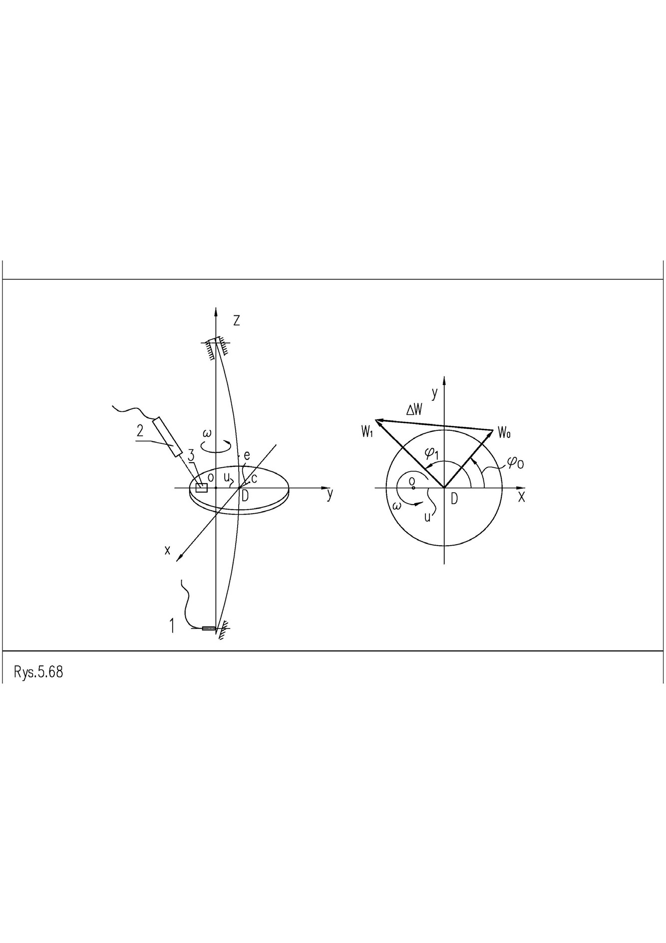
1. vibration sensor,
2. laser sensor with reflected light transmitter and receiver,
3. the film reflecting the laser beam.
The sensor is not attached directly to the target. Due to the assumed linearity of the stiffness characteristics of the disc support, the amplitudes of the signals induced in it are such that they form a triangle like the one that would form where the disc is attached to the shaft.
Modern balancing machines show the measured vibrations as a vector, which has a length and direction of action relative to the adopted angular pitch associated with the rotor. Therefore, on the machine’s screen, the measurement results are called vector indications.
Figure 2 shows a vector that illustrates both vibrations performed with and without a test load. The sensor measures the vibration of the rotating deflection by showing the component in the selected direction.
The basic information contained therein makes it possible to determine that:
a) the rotor is statically unbalanced, since the center of gravity does not lie in the geometric center of the disk, through which the shaft axis passes;
b) each support reacts differently to the attached test load, but it is sufficient to measure the vibration at one arbitrarily selected support to obtain the result in the form of initial unbalance;
c) the force or movement in the lower support is over the entire range of measurements, directly proportional to the deflection of the prone shaft;
d) the sensor picks up the component of force or motion acting in the direction of its main measuring axis.
The last two statements are crucial in using the influence coefficient method. They describe the dynamic response of the support in the location and direction of its action.
The linearity assumption
The coefficient method assumes linearity of the forcing response under given conditions of motion. Let’s define linearity as a simple proportionality between the forcing and the response of the support to this forcing in the form of a force or oscillating motion. Practice shows that susceptibility can be different for small and large forcing. This may be due to the nonlinearity of the support’s stiffness or bending characteristics of the shaft. For a correct result, it should be sufficiently invariant, within the selected range.
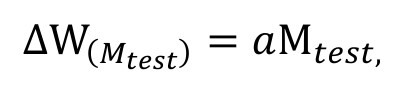
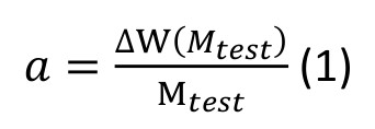
During balancing, the rotor spins, but with the help of the transducer we observe the oscillating motion. The motion or force sensor is fixed stationary with respect to the blade and acts directionally. It registers the motion or rotating force, in-plane, as a component in the selected direction. It has a harmonic waveform. The measurement and calculation module from the harmonic signal creates two harmonic signals, which are components of the vector: sine and cosine. The proportionality factor will be by definition:
In this case:
ΔW(Mtest)
a) is a complex number representing the change in the pointer vector caused by a test weight of Mtest which was mounted on the selected angle,
b) Mtest is written as a complex number because the test weight has characteristics such as the amount of mass (that is, the length of the vector) and angular position relative to the pitch associated with the rotor,
c) a represents the calibration vector (susceptibility coefficient), in the form of a complex number, since it must have the property of both attenuating and amplifying signals, as well as any change phases.
Hence, we get an expression to calculate the value of the coefficient:
or, after inputting the measurement data from both cycles:
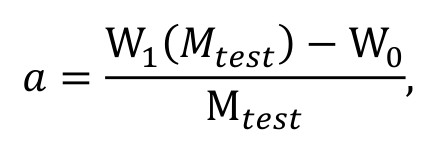
Donde: a = x + iy.
In the equation we have two unknowns: the real and imaginary part of the coefficient a.
We have two scalar equations in which we know the values of the expressions:
a) the mass value of the test weight Mtest and its angular position on the rotor and,
b) vibration amplitudes W0 and W1, corresponding phase angles of motion with and without the test weight.
At this action, the measurement stage ends and the calculation stage begins.
From calibration vector to balancing weight
Suppose that instead of the test weight, with the same coefficient a, we attach a weight of such mass and at such an angular position that its action will cause the vibration to stop. Thus, the load can be called a balancing load Mwyw. For a balancing load, equation (2) takes the form:
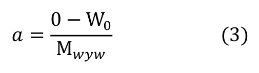
or after transformation:

The vectors in equation (4) have two components. Thus, from the equation we get two scalar equations. On the right side of equation (4) all the values are given, and on the left side we have two unknowns: the value of the weight and its angular position. Using this, the value and angular position of the balancing weight can be determined using the previously determined coefficient and the initial indication of the balancer.
Two worked cases: with and without damping
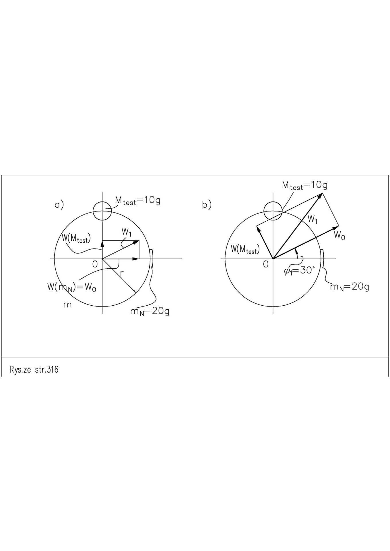
Let’s consider two more situations that can be found during balancing on a test bench with one degree of freedom. These are shown in Figure 3, where:
a) due to the trace damping in the system and the simultaneous subcritical operation of the rotor, there is no phase shift between the forcing (unbalance) and the system response, i.e. deflection (in vibration);
b) with the noticeable effect of damping, at subcritical speed, there is a phase shift between the forcing (unbalance) and the system response, i.e. deflection (in vibration).
The rotors in cases a) and b) are loaded with identical unbalance [20.0 g; 0°]. They are tested with identical weights [10.0 g; 90°].
The acquired measurement results and the corresponding results of the initial unbalance calculation are included in Table 1. In column 1, a has an imaginary part of zero, and in column 2 it is different from zero.
The offset φ1 = 30° is not due to the adoption of a different zero point on the angular scale applied to the rotor. The rotors, shown in columns 1 and 2 (in the table below), have different dynamic properties that are invariant throughout the balancing process. Column 1 in Table 1 corresponds to Figure 3a). The presence of damping in the mechanical system in case b) is the reason for the phase shift of the measured values. The indications W0 and W1 are relative to each other, in both cases separately, in the same ratio of values and are rotated by the same angle.
![Table 1. Balancing without damping (Fig. 3a, column 1) and with a noticeable effect of damping (Fig. 3b, column 2): input data, coefficient k, calibration vector a and balancing weight M_wyw = [20 g; 180°] in both cases.](https://www.ascentialtech.com/wp-content/uploads/2026/10/eq_table1.jpg)
Donde: k is the proportionality coefficient that determines the individual response of the system to the primary load (follows from the figure, that is, from the assumptions), a is the coefficient defined in the coefficient method.
Why constant phase components cancel out
The calculation algorithm eliminates those phase components that are constant throughout the balancing process. As the speed and damping in each stage are the same, the addition to the phase angle due to the dynamic characteristics of the rigid rotor support does not affect the result of unbalance calculations. This is important for balancing in own bearings, where each sensor mount is different in terms of stiffness and damping.