Any structural element of a rotating machine that participates in rotary motion has an axis of symmetry. This axis is also the main mass central axis of inertia, and the mass deviation moments in its direction are zero. If the element actually rotates around it, its mass does not force the motion and thus does not induce forces in its supports.
Mechanical systems that cooperate in rotary motion are usually designed so that their axes of symmetry, when assembled, should also coincide. As a result of trace shape and assembly errors, the actual common axis of rotation of the system most often does not coincide with a selected axis of a component element. Therefore, the common center of gravity of all components of a rotating system does not lie on the actual axis of rotation. Some components may also be attached obliquely, meaning with an angular error. By this, the main mass axis of inertia of the entire rotor lies obliquely with respect to the actual axis of rotation. The position of the actual axis is fixed by the bearing (i.e. by ties). This alignment of the two axes (the main central inertia and the actual spinning axis), with respect to each other, is the source of the motion forcing and additional forces occurring at the support points of the rotor. This forcing is specific to the extent that the amplitude of the forcing force increases with increasing rotation of the rigid rotor and has a constant direction relative to the rotor.
In a rotating machine, the component that is a bond for the rotor and keeps it in the axis of rotation structure is directly exposed to forces from unbalance. These are the bearings mounted on the pivots of the rotor. In them, the rotating inertia forces meet the reactions of the spurs.
The following example shows the destructive effect of forces from unbalance on the life of rolling bearings. This influence is apparent because ball bearings are mechanically resistant to external and lateral forces, among other things. Such lateral forces, which we call inertia forces, arise when the mass of the rotor is accelerated. They counteract this acceleration. Since there is centripetal acceleration in rotary motion, the inertia forces act centrifugally, and their amplitudes depend on the rotational speed.
Modelling the rotor and clutch disc
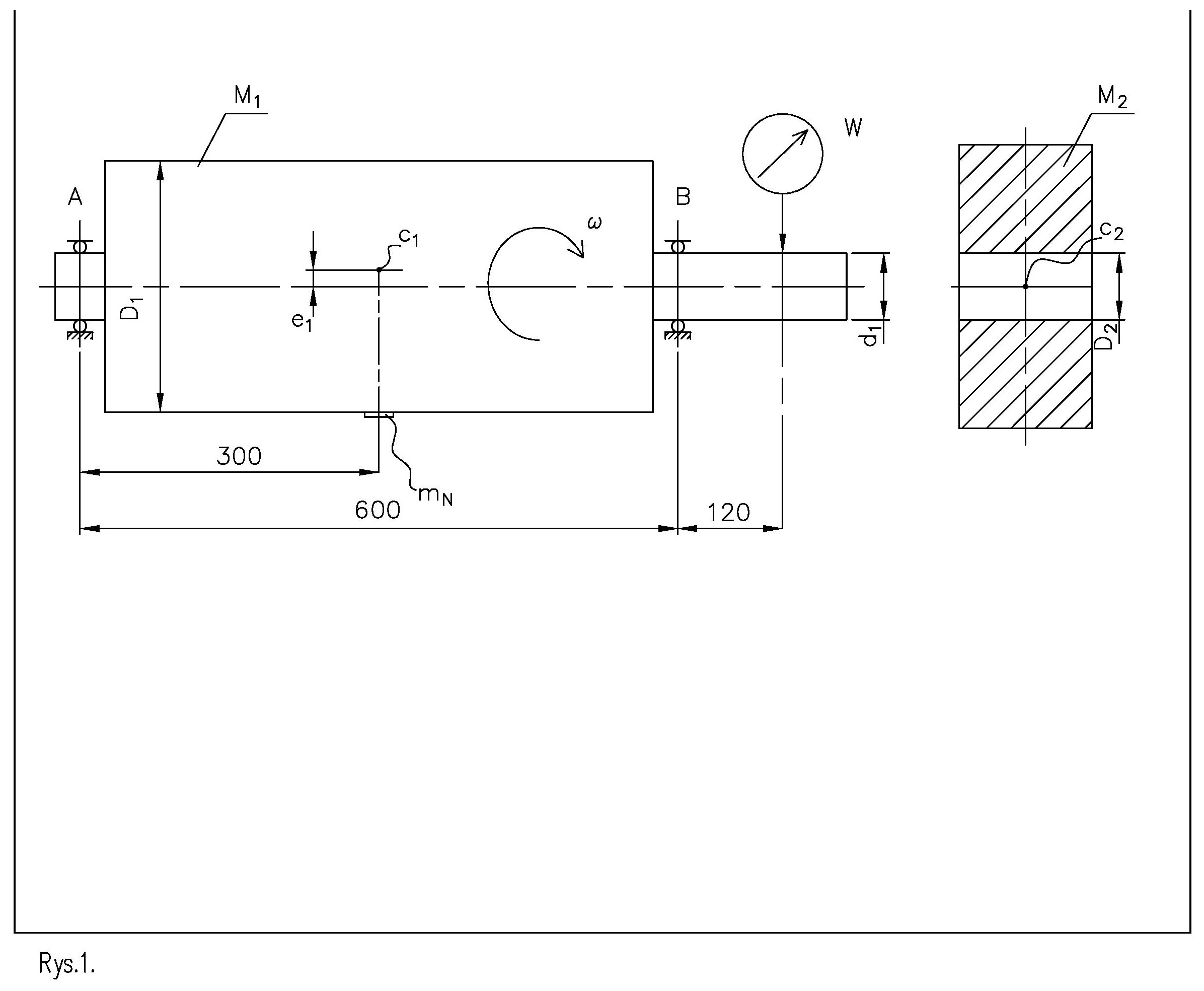
In order to analyze the effect of unbalance on durability and bearing selection, the following model of the rotor-half coupling connection was adopted. The rotor is supported symmetrically with respect to its center of gravity. To simplify the analysis, it was assumed that the rotor material is homogeneous throughout. The measured runout of the rotor journal may be due to shaft curvature or inaccurate machining.
Input data:
M1 = 500 kg (mass of the rotor), M2 = 60 kg (mass of the clutch disc), d1 = 34,984 mm (rotor shaft diameter), D1 = 600 mm (diameter of the outer rotor shaft), D2 = 3,5H7 mm (diameter of the hole made in the clutch disc), W = 24 μm (measured radial runout on the rotor shaft), Lh = 10,000 hours (the number of hours of trouble-free operation assumed by the designer of the rotor device), n = 2,900 rpm (rotor speed).
The rotor has a current balancing protocol stating that it has been balanced in G40 class. The clutch disc has a current balancing protocol stating that it has been balanced in G1 class.
Accepted procedure:
a) Unbalance values will be determined without the use of a balancer.
b) To estimate the value of rotating inertia forces, a path meter will be used to measure the run-out W, as well as measuring the diameter of the shaft d1 and reading the diameter of the hole in the disc D2 from the table.
c) By not being able to measure the value of unbalance with a balancing machine, the composition of forces from unbalance under the least favorable conditions will be assumed. Such conditions correspond to the addition of vectors having the same direction (in reality, the forces can be added in different directions).
It was assumed that the B bearing, which is loaded with higher lateral forces, would be analyzed.
The assumption that a rotor with a mass of M1 = 500 kg has an initial unbalance of G40 means shifting e1 of its center of gravity c1 by the value determined below.
¹ M. Malec: Dynamic balancing of rotors in theory and practice. MM Publications. Bydgoszcz 2022.
Determining the unbalance value
For the determination of the unbalance value, the relationship is used:
𝑁𝑁E = 𝑚𝑚$ ∙ Where: – is rotor unbalance, – balancing accuracy class, – rotational speed, – rotating mass¹.
&,-Q 𝑔𝑔𝑔𝑔𝑔 𝑀𝑀! [𝑔𝑔] 𝑛𝑛 P ()*.
The eccentricity will be determined 𝑚𝑚$ using the value of the corrective weight that would balance the rotor if it were seated at radius .
Relationship (1) after transformation for unbalance G40 and rotation n = 2900 obr/min has the form:
𝜋𝜋∙𝐷𝐷! ∙𝑛𝑛= 60 ∙5 ∙10. ∙40 𝑚𝑚$ = 60 ∙𝑀𝑀! ∙𝐺𝐺 𝑚𝑚$ Where : is a mass centered at a point, seated on a radius , giving an unbalance .
Use the relationship of the equality of the static moments of the entire rotor on the eccentricity and the balancing correction weight seated on the diameter:
%!
“
𝑀𝑀! ∙𝑒𝑒! = 𝑚𝑚$ ∙𝐷𝐷!
From here:
𝑒𝑒! = 𝑚𝑚$ ∙𝐷𝐷!
2 ∙𝑀𝑀! = 219.6 ∙600 G = NEπn 30M! (1)
” [𝑔𝑔𝑔𝑔𝑔𝑔]𝑀𝑔𝑚 “
%!
𝐺𝐺 𝐺P ‘ Q𝑁 && e!
%!
“
3.14 ∙600 ∙2900 = 219.6 𝑔𝑔, %!
NE “
𝑒𝑒!
2 (2)
2 ∙5 ∙10. = 0.131 𝑚𝑚𝑚𝑚= 131 𝜇𝜇𝜇𝜇 Hence, the radial runout to be measured on the cylindrical surface:
𝑤𝑤! = 2𝑒𝑒! = 0.262 𝑚𝑚𝑚𝑚= 262 𝜇𝜇𝜇𝜇 The component forces acting on the bearing are:
a) F1 constant in value and direction resulting from the weight of the rotor and coupling,
b) F2 rotating, resulting from the unbalance of the rotor,
c) F3 rotating, resulting from the unbalance of the clutch disc caused by the eccentricity of its attachment to the rotor shaft (note: it is assumed that the clutch disc was balanced and its residual unbalance has a small value that can be ignored).
The three component forces on the bearing
The force of gravity on the rotor is always directed downward. Inertia forces caused by unbalance rotate with the rotor. Therefore, the bearing is loaded with a variable force as to value and direction. The value varies from a minimum, which is to a maximum, which is The direction of the resultant action is variable in the range of . It was assumed here that the coupling was fixed on the shaft at the most unfavorable relative arrangement of clearances and, consequently, inertia forces, due to the lack of control of the angular position of the coupling and rotor unbalance.
𝐹𝐹’0& = 𝐹𝐹! −𝐹𝐹” −𝐹𝐹/.
𝐹𝐹’0& = 𝐹𝐹! + 𝐹𝐹” + 𝐹𝐹/.
∓𝜑𝜑 Determination of forces acting on the bearing B.
𝐹𝐹” = 1 2 [𝑀𝑀!𝜔𝜔”𝑒𝑒!] = 1 2 _𝑀𝑀! `𝜋𝜋𝜋𝜋 30a “
Clearance in the clutch disc mounting
The calculation of the force will be preceded by a dimensional analysis of the kinematic pair that is the shaft and clutch disc.
Practice shows that components mounted on rotor shafts are a source of additional unbalance and thus a source of additional vibration of the aggregates. The behavior of the clutch disc after it is mounted on the rotor shaft should be initially analyzed.

∅35𝐻𝐻7 = 35!
𝐹𝐹! = 𝑀𝑀! ∙𝑔𝑔 2 = 500 ∙9.81 2 = 2452 𝑁𝑁 𝑒𝑒!b = 1 2 c5 ∙10. ∙d3.14 ∙2900 30 e “
0.131f = 3017 𝑁𝑁 “!.!$%𝑚𝑚𝑚𝑚.
The clutch disc can be fixed on the rotor arbitrarily, but within its clearance, while the clearance can be cleared at any random angle in the plane perpendicular to the axis of rotation. According to the rules, we assume the worst case: the runout of the shaft and the maximum deviation of the hole execution add up in the same direction.
The rotor, in the planes in which the bearings are mounted, rotates relative to the actual axis of rotation 1. The geometric axis of the end of the rotor shaft is the axis 3. The main central axis of inertia of the coupling disc, along with the center of gravity c2, is the axis 2.
Eccentricity of the center of gravity position of the clutch disc resulting from the transverse runout of the shaft:
𝑒𝑒$ = 𝑊𝑊 2 = 0.024 2 = 0.012 𝑚𝑚𝑚𝑚= 12 𝜇𝜇𝜇𝜇.
Eccentricity resulting from making the shaft below the nominal value and the hole in the upper deviation:
𝑒𝑒& = ∅'() −𝑑𝑑* 2 = 35.025 −34.984 2 = 0.0205 𝑚𝑚𝑚𝑚= 20.5 𝜇𝜇𝜇𝜇.
Total eccentricity of clutch disc mounting on rotor shaft:
𝑒𝑒+,’ = 𝑒𝑒$ + 𝑒𝑒& = 0.012 + 0.0205 = 0.0325 𝑚𝑚𝑚𝑚= 32.5 𝜇𝜇𝜇𝜇.
Eccentricity resulting from off-center attachment of clutch disc:
𝑁𝑁7 = 𝑀𝑀$ ∙𝑒𝑒+,’ = 60 ∙10& ∙0.0325 = 1950 𝑔𝑔𝑔𝑔𝑔𝑔.
Force from the clutch disc eccentricity
The force F3 is determined by the relationship:
𝐹𝐹/,) = 𝑁𝑁E ∙𝜔𝜔” = 𝑀𝑀”𝑒𝑒’0&𝜔𝜔” = 6 ∙102 ∙0.0325 ∙d3.14 ∙2900 The actual force on the bearing B, using the equation of the sum of moments with respect to, for example, the point A shown in the figure 1, is:
𝐹𝐹/ = 215.5 𝑁𝑁 In the case in which after the rotor manufacturing process and before balancing its unbalance corresponds to the G40 balancing accuracy class, with uniform distribution of the bearing load from the rotor weight we have the following values of the component forces loading the bearing B:
Table 1. forces acting on the bearing B at n = 2900 o br/min and G40 initial unbalance.

= 179.6 𝑁𝑁 30 e G40 n = 2900 rpm F1 = 2452 N F2 = 3017 N F3 = 215.5 N When selecting bearings according to the catalog, e.g. SKF, under rotating load conditions, the value of the load variation factor should be determined and included in the equation for determining the average load:
𝐹𝐹& = 𝑓𝑓&(𝐹𝐹! + 𝐹𝐹” + 𝐹𝐹/)
Selecting the bearing: the fm coefficient
To determine this coefficient, plot the r𝑓𝑓& function of variation of the parameter as a function of the values of the rotating forces F2 and F3 Chart 1².
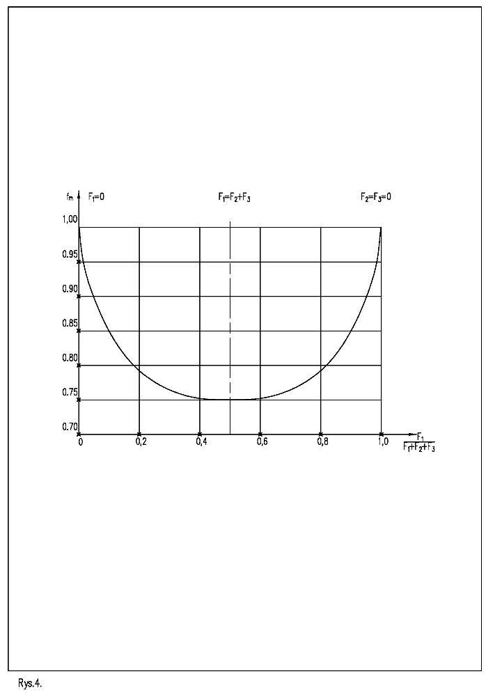
To determine the value of the fm coefficient, perform an auxiliary calculation:
𝐹𝐹! 𝐹𝐹! + 𝐹𝐹” + 𝐹𝐹/ = 2452 2452 + 3017 + 215 = 0.43 𝑓 For the calculated value read from the catalog’s chart 1: fm = 0.77.
² Roller bearing catalog r𝑓𝑓& 𝐹 For this value fm, the average bearing load, according to the catalog, is:
𝐹𝐹& = 𝑓𝑓&(𝐹𝐹! + 𝐹𝐹” + 𝐹𝐹/) = 0.77(2452 + 3017 + 215) = 4376 𝑁𝑁 𝑁(2)
Assumptions for required bearing life
Making assumptions about the required bearing life:
a) the forces acting on the bearing have a radial direction from where the equivalent dynamic load is: P = Fm,
b) it is assumed that the bearing should operate for hours.
Using the chart for calculating bearings, you can check the effect of the value of the lateral forces:
c) it is assumed that the bearing should operate Lh = 10,000 hours
d) the reduction of the operating time of the used bearing due to additional rotating forces.
Regarding c., select a bearing by finding the nominal dynamic load capacity C.
Some notes on the construction of nomograms.
How the nomograms are built
Nomograms were developed when rotor designers used simple calculation tools. Their current importance lies mainly in a good visualization of the bearing selection process.
The word nomograms is used in the plural, because the vertical alignment of the axes: P[N] & C[N] with respect to the other axes may be slightly shifted on charts made by different bearing manufacturers. It depends on the bearing performance obtained. Axes: Lh[h], L[mln rpm.] & n[rpm] are uniquely related to each other by rotor kinematics. For example: in 100 hours of operation at 2500 rpm, the rotor will make 100•2500•60=15 million revolutions. These three axes are arranged with respect to each other in such a way that any straight line connecting the selected rotations with the assumed number of hours of failure-free operation of the bearing will give the correct result of the above multiplication on the L[mln rpm] axis.
The position and scales of the other axes are derived from the performance of the bearings of the respective manufacturer. They are so located and stretched, along their lengths, that another straight section, passing through the previously determined point on the L[million rpm] axis, will connect the value of the total lateral forces in the bearing, shown on the P axis, with the determined value of C determining the choice of bearing size³.
Adopting a logarithmic scale shortens the axis lengths.
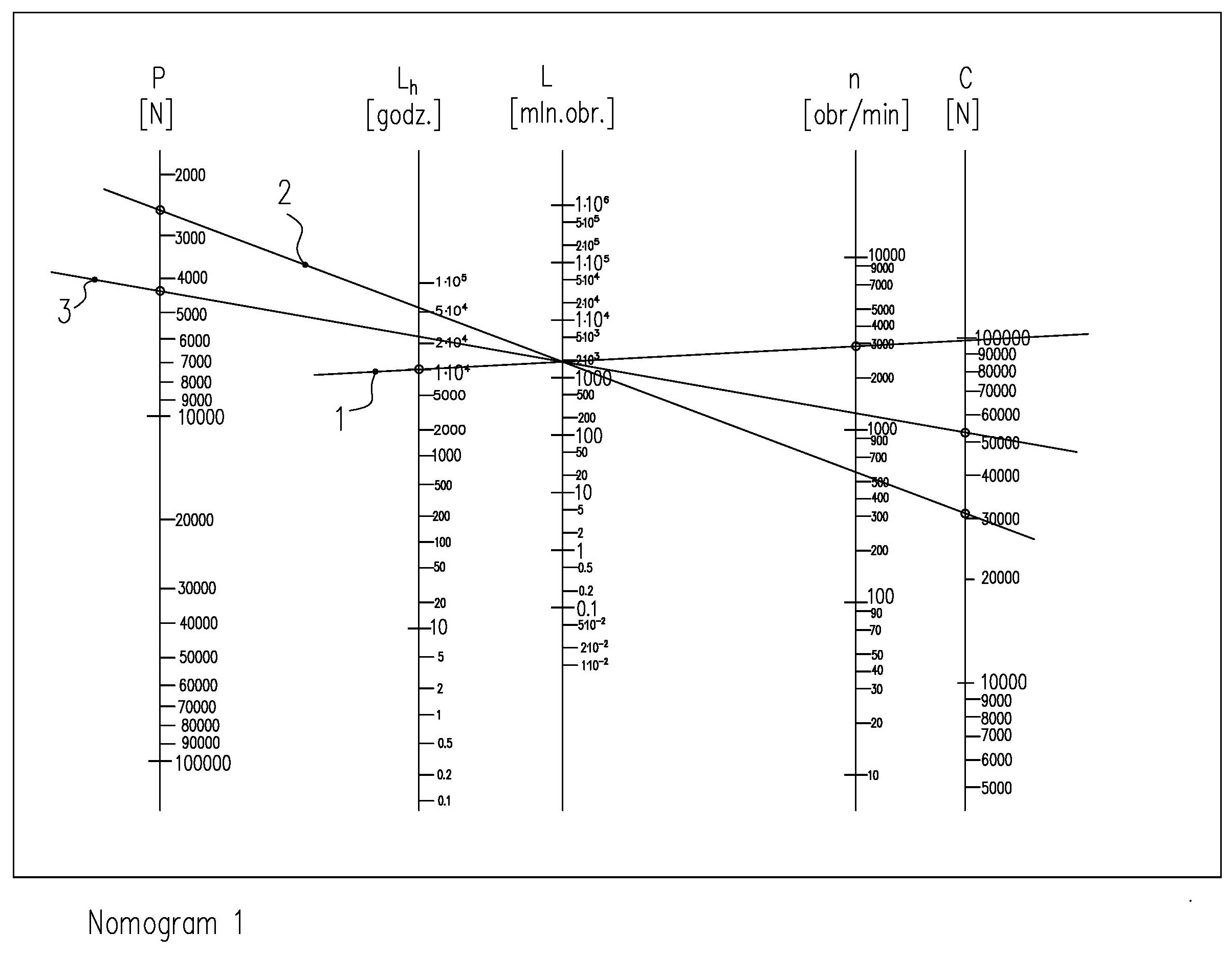
In nomogram 1, straight line 1 is an auxiliary line that, for the assumed number of operating hours Lh and at ³ Roller bearing catalog the specified rotor speed n=2900 rpm, determines the number on the L-axis that determines the number of revolutions counted in millions in the assumed time. The straight line 2 intersecting the determined point on the L-axis and simultaneously passing through the point determining the static load of the bearing (2452 N) determines at the other end the required nominal static load capacity of the bearing C. Here it amounts to about 32 kN. This is the load capacity for the static case.
Straight line 3, passing through the point determined by line 1 on the L-axis and through the point determining the total static and dynamic load Fm = P, written in equation (2) amounting to 4376 N, determines the new required nominal dynamic bearing capacity of the bearing. Here it amounts to about 54 kN.
Nomogram 1. Selecting the nominal dynamic bearing capacity C for the assumed number of operating hours Lh and the equivalent dynamic load P.
Conclusion: Adding to the forces, coming from the weight of the rotor, the forces coming from the initial unbalance of the rotor and the unbalance caused by the eccentricity of the attachment of the coupling disc to the shaft, the required nominal bearing capacity C determined for static forces increased by about 67%. The presence of unbalance on the Nomogram 1.
rotor puts additional load on it to an extent that cannot be ignored for the accepted data. The load of rotating forces can result in overloading and destruction of the bearing. It will also shorten its failure-free life.
Recalculating bearing life under added forces
Ad d. Determination of the new operating time Lh for the applied bearing loaded with additional rotating forces F2 & F3 at the assumed nominal dynamic bearing capacity C.
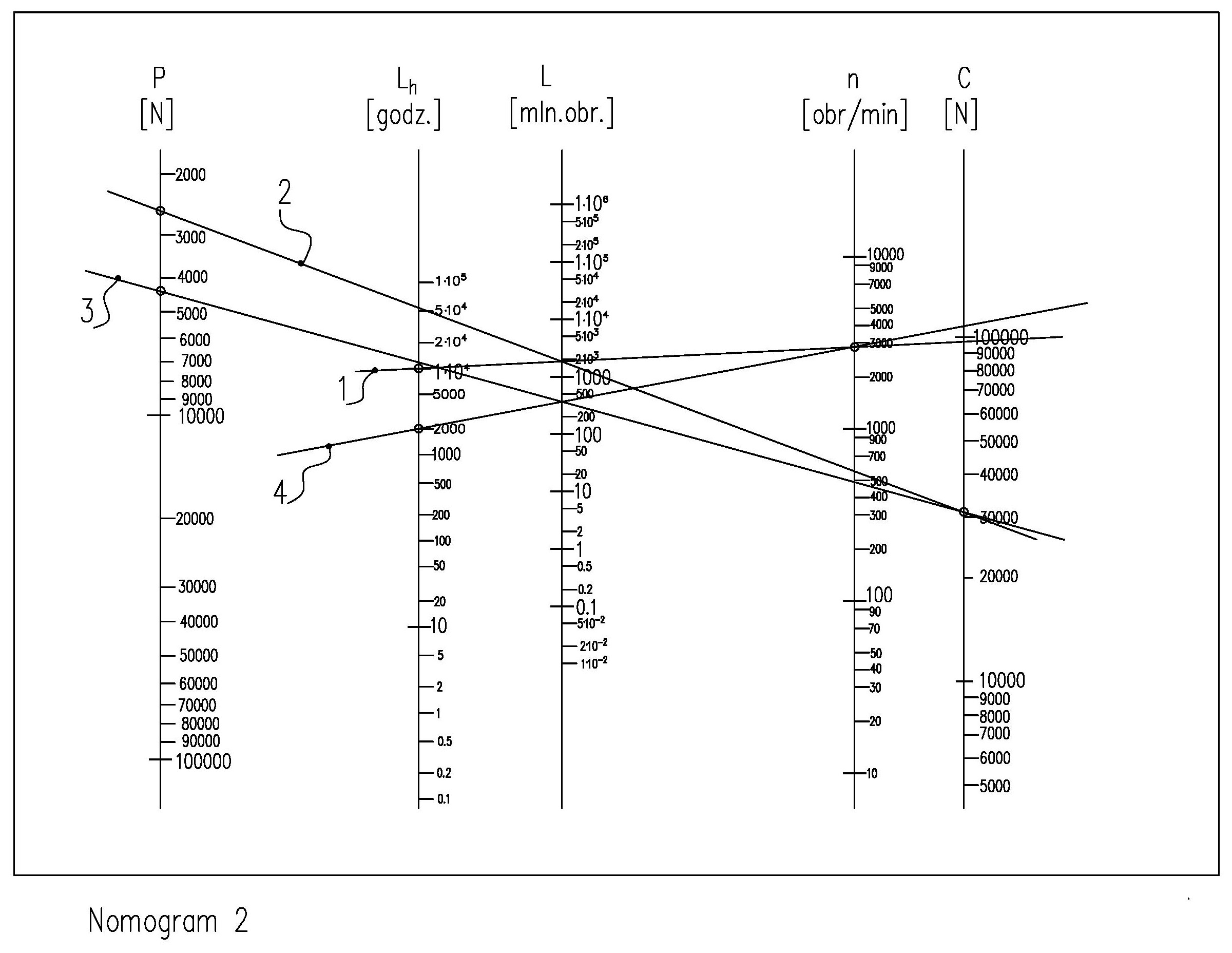
In nomogram 2, straight lines 1 and 2 determine the same values as in monogram 1.
Line 3 is drawn differently. The purpose of the procedure is to determine a different nominal life L measured in millions of revolutions of the selected bearing loaded with rotating forces in addition to static forces. The line connects the total value of all forces: static and rotating, converted to an average value of Fm = 4376 N, with the previously determined only for static loading nominal load capacity C. This straight line on the L-axis determines the new value of the number of revolutions counted in millions of revolutions. Straight line 4, combining this new value on the L-axis with the previously assumed revolutions per minute, determines on the Lh axis the new number of hours of failure-free operation of the bearing.
Nomogram 2. Determination of the new operating time Lh for the applied bearing loaded with additional rotating forces F2 & F3 at the assumed nominal dynamic bearing capacity C.
Conclusion: As a result of the occurrence of additional rotating forces from the unbalance of the rotor and the coupling element, the failure- free operating time decreased from Nomogram 2.
10,000 hours, with the rotor balanced and the coupling rebalanced after its installation on the shaft, to about 2,000 hours with the rotor and the coupling unbalanced.
Selecting a larger sized bearing whose nominal dynamic load capacity C will allow it to carry the load from unbalance does not solve the problem. It will increase the dimensions of most rotating components. This will also increase their initial unbalance, which is due to the current accuracies used in manufacturing. An effective solution is balancing.